Excel has a lot of functions that you can use including VLOOKUP. If you are considering using some of these functions and formulas, you need to know more about them. VLOOKUP in Excel is one of the formulas that you can use when you have large amounts of data.
What Is VLOOKUP In Excel?
As the name suggests, VLOOKUP is a lookup function in Excel which will retrieve data from a specified column in a table. The V in the name stands for vertical which is the direction that the formula works. This means that you can only use this formula to look up data by column and not by row.
When using VLOOKUP, you will be looking up a value in a set table of data by matching a value in the initial column of the table. There is no way to change the formula to match data in any other column other than the first one. However, it is possible to use approximate, partial and exact matching.
When using this function, it is important to note that it only looks right. This means that the retrieved data will need to be in columns to the right of the initial column used in the function. The data that is retrieved will be based on column number and you need to remember this when using the function.
When To Use VLOOKUP
There are many situations when you would need to use VLOOKUP. However, the most common is when you have a table of data and need to retrieve values from columns based on the information in the initial column. The initial column will need to have unique identifiable values which can be used to run the function.
One of the most common situations for this function to be used is when you have ID numbers linked to additional data. This could be when you have three-digit ID numbers linked to information such as email addresses, names and physical addresses. In these situations, you will be able to use the function to look up the ID number and retrieve the email address, physical address or name linked to it. It is important to note that you will only be able to retrieve one piece of information per VLOOKUP.
How To Use VLOOKUP
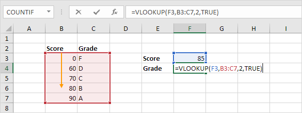
When it comes to using the function, you will need to understand the syntax. The syntax for this function is VLOOKUP (value, table, col_index, [range_lookup]). Each part if the syntax needs to be understood and the correct values inserted.
The value in the syntax will be the value that you want to look up in the initial column such as the ID number. The table is the defined range of rows and columns that the function should use to find the value. The col_index is the column that you want the data to be retrieved from. This will be a number for the column starting from 2.
The last part of the syntax relates to the type of match you want. This is an optional part of the syntax. Using TRUE will ensure approximate matches and is the default while FALSE will be an exact match.
You can enter all of the information you need through the formula wizard. To get to this, you will need to go to the formula tab and choose insert function. You will need to find VLOOKUP and use the wizard to enter all of the data that you need.
VLOOKUP in Excel is one of the formulas that you may need to use. This formula will retrieve data through a vertical search using columns. If you want to retrieve data by rows, you will need to use HLOOKUP.
